Spectral Clustering in J

With Examples from Quantitative Neuroscience

In my never ending quest to understand hard, but useful stuff, I’ve been learning the Programming Language J. J is an array oriented language in the APL family. Matlab is a related language, but its APL-ness is quite attenuated compared to J. I know Matlab already, having used it quote extensively as a research scientist, so J is not utterly alien, but unlike Matlab, which presents a recognizable syntactic face to the user, J retains an APL-like syntax.

As you will see, this presents challenges. The best way to learn to use a tool is to use it, so I thought I would take the opportunity to investigate a clustering technique which would have been useful to me as a grad student (had I known about it): Spectral Clustering.

Spectral Clustering¹ refers to a family of clustering approaches which operate on the assumption that local information around data points is more useful for the purposes of assigning those points clusters than is their global arrangement. Typical clustering techniques, like k-means, make the assumption “points in a cluster will be near to eachother.” Spectral clustering relaxes that assumption to “points in a cluster will be near to other points in their cluster.”

We will develop the spectral clustering algorithm and then apply it to a series of more interesting data sets.

Part 1: 1d Gaussian Clusters

We are going to work on exploring spectral clustering. In order to do that we need something to cluster. Our first data set will be trivial: made by combining two sets drawn from different normal distributions².

load 'utils.ijs'
load 'km.ijs'
require 'graphics/plot'
require 'numeric'
require 'viewmat'
require 'math/lapack'
require 'math/lapack/geev'

clusterSize1 =: 100
e1d1 =: (0 0.01) gausian clusterSize1
e1d2 =: (13 0.01) gausian clusterSize1

e1labeled =:  (((clusterSize1$0),(clusterSize1$1))) ,: (e1d1, e1d2)
e1data =: 1 { e1labeled
e1labels =: 0 { e1labeled


NB. show the histogram of the data
NB. (_6 6 200) histPlot e1data

The commented line produces the following plot:

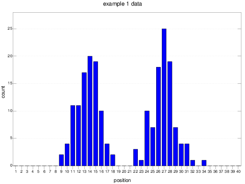
This kind of data is trivial to cluster with an algorithm like k-means³.

kmClustering  =: 2 km (((# , 1:) e1data) $ e1data)

+/ (kmClustering = e1labels)

Should give ~ 200, unless something unusual happens.

As I suggested in the introductory section, the magic of spectral clustering is that it works on a representation of data which favors local information about the relationships between objects. Hence we will need to create some sort of connectivity graph for our data points. There are lots of approaches, but the upshot is that i,j in our connectivity matrix must tell us whether it is likely that point i and point j are in the same cluster.

For this simple example, we will just use the Euclidean distance between points and a threshold: anything lower than the threshold is connected and anything higher is not.

NB. d is the distance between two vectors of equal dimension
d =: %:@:+/@:*:@:([ - ])

NB. ds is the table of all pairwise distances where each argument is a
NB. list of vectors.
ds =: d"(1 1)/

NB. convert a list of points to a list of 1d vectors
l2v =: (#@:],1:) $ ]

NB. ds for lists of points
ds1d =: l2v@:] ds l2v@:]

NB. the table of all distances of x
dof =: ] ds ]

NB. the same except for a list of points
dof1d =: ] ds1d ] 

connections1d =: [ <~ dof1d@:]

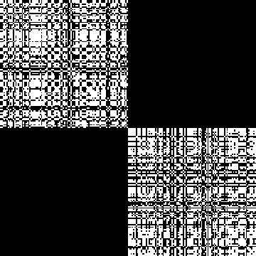
e1connections =: 1.0 connections1d e1data

NB. viewmat e1connections

The connections matrix looks like:

Spectral clustering operates on a Matrix called the Graph Laplacian which is related to the connectivity matrix. To get the laplacian matrix L we subtract the connectivity matrix from something called the degree matrix. Explained clearly but without interpretation, the degree matrix is just the sum of all connections for a given vertex in our graph, placed on the diagonal.

calcDegreeMat =:  (eye@:#) * +/"1 

The degree matrix just tells you how connected a given vertex is. To get the Laplacian Matrix you subtract the connectivity matrix from the degree matrix. This is conveniently defined in J:

calcLap =: calcDegreeMat - ]

For our first data set, this Laplacian looks like:

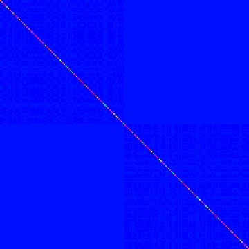
Brief meditation will explain why the components of this matrix representing inter-object connections are so faint compared to those on the diagonal: the rank of each vertex in the graph is always larger than its connections, being the sum thereof.

Now that we have the Laplacian I will perform:

Spectral Clustering

The paper A Tutorial Introduction to Spectral Clustering, describes a family of spectral clustering strategies. We will implement just the first.

It involves the steps:

1. Find the graph Laplacian for your system
2. Find its eigenvalues and eigenvectors
3. Sort the latter by the former, in ascending order
4. Arrange the vectors as columns of a matrix
5. truncate that matrix to a small number of columns, corresponding to the smaller eigenvalues.
6. treat the rows of the resulting matrix as vectors.
7. perform clustering, say k-means, on those vectors.

We can denote these succinctly in J:

eigensystem =: monad define 
  raw =. geev_jlapack_ y
  ii =. /:@:>@:(1&{) raw
  lvecs =. |: (ii { |: (0 unboxFrom raw))
  vals =. ii { (1 unboxFrom raw)
  rvecs =. |: (ii { :| (2 unboxFrom raw))
  lvecs ; vals ; rvecs  
)

eigenvectors =: >@:(0&{@:eigensystem)
eigenvalues =: >@:(1&{@:eigensystem)

takeEigenvectors =: |:@([ {. |:@:])

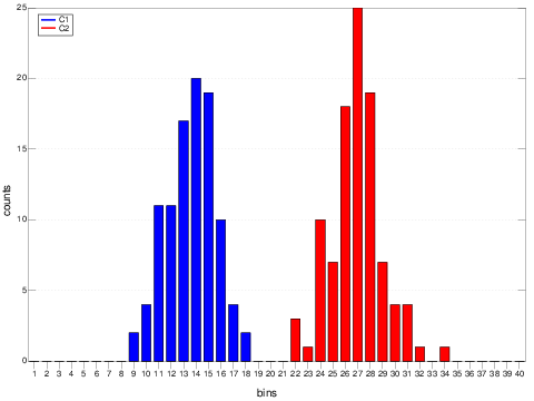
e1clustering =: 2 km takeEigenvectors eigenvectors e1Lap

(+/ e1clustering = e1labels) NB. should be about 200

A boring, if resounding, success.

Example 2: Concentric Clusters

Consider the following data:

rTheta =: (([ * cos@:]) , ([ * sin@:]) )"(0 0)
e2clusterSize =: 100
e2d1 =: ((1,0.1) gausian e2clusterSize) rTheta ((0,2p1) uniform     e2clusterSize)
e2d2 =: ((4,0.1) gausian (2*e2clusterSize)) rTheta ((0,2p1) uniform     (2*e2clusterSize))
e2data =: e2d1, e2d2

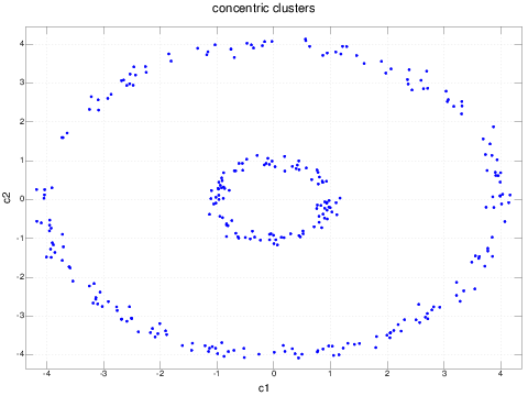
This is the sort of data set which is pathological for clustering procedures which work in the original coordinates of the data. Even traditional dimension reducing techniques like principal component analysis will fail to improve the performance (in fact, the principal components of this data set are analogous to x and y, modulo a rotation).

We could, of course, realize by inspection that this problem reduces to the first example if the angular component is thrown away and we cluster on the radial component only.

However, in general, we are working with data in n dimensions and such simplifications may not be apparent to us. Hence, we will proceed with this example set.

Again, we produce the connectivity matrix by simple c_i,j = d_i,j < epsilon.

e2connections =: 1 connections e2data 
e2Lap =: calcLap e2connections
e2ids =:  2 km 2 takeEigenvectors eigenvectors e2Lap

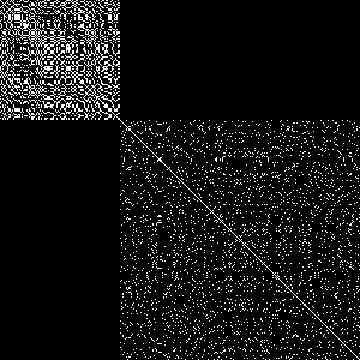
As we physicists like to say: now we just turn the crank:

e2Lap =: calcLap e2connections
e2ids =:  2 km 2 takeEigenvectors eigenvectors e2Lap

And we can plot these points labeled by ID:

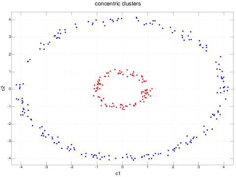
Pretty neat - we have successfully clustered a data set which traditional techniques could not have dealt without, and without manually figuring out a transform the simplified the data set.

Example 3: Neural Spike Trains

My interest in spectral clustering goes back to my graduate research, which involved, among other things, the automatic clustering of neural data. Neurons, in animals like us, anyway, communicate with one another using brief, large depolarizations of the voltage across their cell membranes. Neuroscientists call these events spikes and they literally look like large (~80 mV) spikes of voltage in the recording of the voltage across a cell membrane. These spikes travel down the neuron's axon and are transmitted through synapses to other neurons. There are other forms of communication between neurons, but it is generally assumed that spikes underly much of the computations that neural networks perform.

Spikes are short (1-2 ms) and firing rates are generally low on this time scale, with a typical inter-spike period of 10-100 ms (depending a great deal on the inputs to the neuron). In order to understand how neurons work, neuroscientist repeat a stimulus over and over again and record the spike times relative to the beginning of the experiment.

This results in a data set like:

33.0  55.2  80.0
30.0  81.1
55.2  85.9

Where rows are trials and each number is a spike time for that trial. In J we can read this data as padded arrays:

spikes =: asArray 0 : 0
33.0  55.2  80.0
30.0  81.1
55.2  85.9
)

And J will pad it out with zeros.

 33   55.2   80
 30   81.1   0
 55.2 85.9   0

Under certain circumstances, during such experiments, neurons generate a small number of distinct spiking patterns. Assuming that these patterns may be of interest, much of my research focused on extracting them automatically. That is: given a data set of spike trains, extract the clusters of similar trains.

Unfortunately, spike trains are not vectors and so there is no convenient euclidean distance measure one can easily apply to them. Luckily Victor and Purpura (1996) developed an edit-distance metric on spike trains by analogy to similar metrics other, non-vector, data (like gene sequences).

The Victor-Purpura Metric defines the distance between two spike trains as the minimum cost of distorting one spike train into the other using just two operations: sliding spikes in time to line up or deleting/adding spikes. The cost of sliding spikes in time is has the parameterized cost q*dt where dt is the time difference, and the cost of adding or removing a spike is one.

The algorithm to find the minimum such distortion can be easily implemented:

vpNaive =: adverb define 
  :
  'q' =. m
  's1' =. nonzeros x 
  's2' =. nonzeros y
  'n1' =. #s1
  'n2' =. #s2 
  if. n1 = 0 do.
    n2
  elseif. n2 = 0 do.
    n1
  elseif. 1 do.
    'h1' =. {. s1
    'h2' =. {. s2
    'movecost' =. q * abs (h1-h2)
    if. movecost < 1.0 do.
      'restcost' =. ((}. s1) (q vpNaive) (}. s2))
      restcost + movecost 
    else.
      'restcost' =. ((}. s1) (q vpNaive) (}. s2))
      restcost + 1
    end.
  end.
)

although much more efficient implementations are possible. For our purposes, this will suffice.

With this definition, we can produce the similarity matrix for a given q using this J adverb:

spikeDistances =: adverb define   
  y ((m vpNaive)"(1 1) /) y
)

The choice of q is an important issue which we will neglect for now. See my doctoral thesis for insight into this question. The one sentence upshot is that q should generally be chosen to maximize the information content in the resulting similarity matrix.

Now let's create an example data set consisting of two distinct firing patterns. A firing pattern consists of a mean time for each "event" in the pattern, plus that events "reliability," which is the probability that a spike actually appears in an event. An event may be localized at a very specific time, but spikes may only sometimes appear on a given trial in that event.

Consider:

NB. This produces a fake spike data set of Y trials with events
NB. specified by means, stds, and reliabilities, passed in as a
NB. rectangular matrix.
makeSpikes =: dyad define 
  'means stds reliabilities' =. x
  'n' =. y

  spikes =. (n,#means) $ means 
  spikes =. spikes + ((n,#stds) $ stds)*(rnorm (n,#stds))
  spikes =. spikes * ((runif (n,#reliabilities))<((n,#reliabilities) $   reliabilities))
  nonzeros"1 spikes
)

This function takes a description of the pattern, like:

e3pattern1 =: asArray 0 : 0 
  10 20 30
  1  1.5  1.5
  0.9 0.9 0.6
)

e3pattern2 =: asArray 0 : 0
  15 40
  1  1
  0.8 0.8
)

And returns a data set of N trials:

NB. Now we use makeSpikes to generate the actual data sets.
e3spikes1 =: e3pattern1 makeSpikes 50
e3spikes2 =: e3pattern2 makeSpikes 50

NB. and the utility `concatSpikes` to combine them.  This just makes
NB. sure the zero padding works.
e3spikes =: e3spikes1 concatSpikes e3spikes2

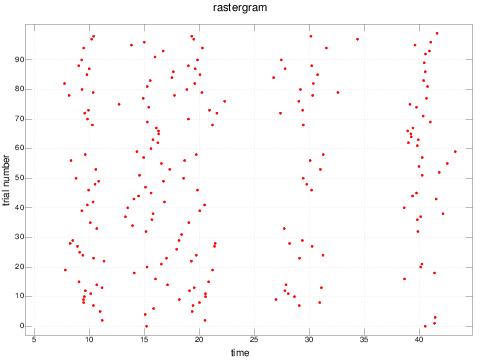
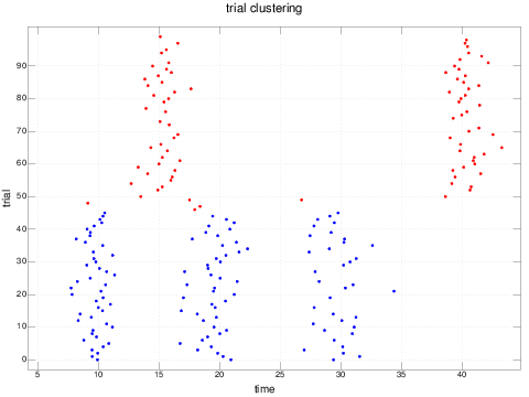
We can plot this data in the traditional fashion, as a "rastergram," where each spike is plotted with its time as the x-coordinate and its trial as its y-coordinate:

rastergram e3spikes

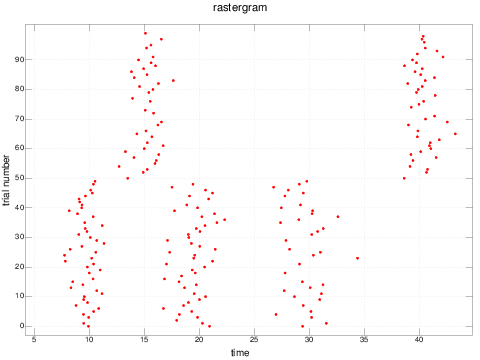
It is interesting to note how difficult it can be to see these patterns by visual inspection if the trials are not sorted by pattern:

rastergram shuffle e3spikes

Now let's cluster them:

NB. We produce the distance matrix
e3distances =: (0.8 spikeDistances) e3spikes

We use thresholding to generate our connectivity matrix:

e3connections =: e3distances < 2

And we turn the crank:

e3Lap =: calcLap e3connections
e3evs =: eigenvectors e3Lap
e3clustering =: 2 km (2 takeEigenvectors e3evs)

Finally, we can color code our rastergram by clustering:

pd 'reset'
pd 'type dot'
pd 'color blue'
pd 'title trial clustering'
pd spikesForPlotting (e3clustering = 0) # e3spikes

pd 'color red'
pd (#((e3clustering=0)#e3spikes)) spikesForPlotting ((e3clustering =   1) # e3spikes)

pd 'xcaption time'
pd 'ycaption trial'

pd 'show'

---

Footnotes

¹

A Note On Simpler Clustering Algorithms

One can appreciate a family of clustering approaches by starting with Expectation Maximization: a two step iterative process which attempts to find the parameters of a probability distribution assumed to underly a given data set. When using this approach for clustering, one assumes that the data has hidden or missing dimensions: in particular, a missing label assigning each point to a cluster. Given some guess at those labels, you can calculate the parameters of the distribution. Using this estimate, you can modify the guess about the hidden labels. Repeat until convergence.

In practice, simplification over the general case can be found by assuming that the distribution is a "Gaussian Mixture Model," just a weighted combination of n-dimensional Gaussian distributions. Further simplifications manifest by applying ad-hoc measures of cluster "belonging" based on just the mean of each cluster (see fuzzy clustering) and finally just by assuming that objects belong to the cluster to which they are closest (as in k-means).

In all of these simplifications clustering refers to some sort of centroid of the clusters as a way of estimating which object belongs to which clusters. But some data sets have clusters which are concentric. For instance, if one cluster is points between 10 and 20 units from the origin and another is points between 50 and 60 units from the origin.

In this case, all such attempts will fail unless the space is transformed. Spectral clustering transforms the space by considering topological information: that is, what objects are near or connected to what other objects, and throwing away large scale information.

In the concentric example above, the thing that all points in each cluster have in common is they are near other points in their cluster. When our distributions have the property that the distance between some two points in cluster A may be greater than the distance between some point in A and some point in B, the spectral clustering gives a nice mechanism for identifying the clusters.

²

Utilities

Throughout the above I refer to the occasional utility. Here are the definitions.

load 'stats/distribs'
load 'numeric'
load 'graphics/plot'

gausian =: dyad define
 'm s' =. x
 m + (s*(rnorm y))
)

uniform =: dyad define 
 'mn mx' =. x
 mn + ((mx-mn)*(runif y))
)

shuffle =: (#@:] ? #@:]) { ] 

hist =: dyad define 
  'min max steps' =. x
  'data' =. ((y<min) * (y>max)) # y
  'quantized' =. >. (steps * ((data - min) % (max-min)))
  'indexes' =. i. steps
  'stepSize' =. (max-min)%steps
  1 -~ ((indexes, quantized) #/. (indexes, quantized))
)


curtail =: }: 

histPlot =: dyad define 
  h =. x hist y 
  'min max nsteps' =. x 
  halfStep =. (max-min)%(2*nsteps)
  'plotXs' =. halfStep + steps (min, max, nsteps)
  'xcaption position; ycaption count; title example 1 data' plot (curtail plotXs) ; h 
)


unboxFrom =: >@:([ { ])

dot =: +/ . *

dir =: monad define 
  list (4 !: 1) 0 1 2 3
)

xyForPlotting =: (0&{ ; 1&{)@|:

ten =: monad define 

10

)

abs =: (+ ` - @. (< & 0))"0

nonzeros =: ((>&0@:abs@:]) # ])

asArray =:  ". ;. _2

concatSpikes =: dyad define
  maxSpikes =. (1 { ($ x)) >. (1{($y))
  pad =. (maxSpikes&{.)"1
  (pad x), (pad y)
)

spikeIndexes =: |:@:(( 1&{@:$@:], #@:[) $ (i.@:#@:]) )
spikesForPlotting =: verb define 
  0 spikesForPlotting y
  :
  spikes =. ,y
  ii =:  ,spikeIndexes y
  nzii =. -. (spikes = 0)
  (nzii # spikes) ; (x+(nzii # ii))
)

rastergram =: monad define
  pd 'reset'
  pd 'type dot'
  pd 'color red'
  pd 'title rastergram'
  pd 'xcaption time'
  pd 'ycaption trial number'
  pd spikesForPlotting y
  pd 'show'
)

offsetY =: ] + ((#@:] , 1&{@:$@:]) $ (0: , [))

eye =: (],]) $ ((1: + ]) take 1:)

asOperator =: adverb define 
  m dot y
)

³

K-Means

An implementation of k-means in J is comically terse, even in an exploded, commented form:

NB. This file contains an implementation of k-means, a clustering
NB. algorithm which takes a set of vectors and a number of clusters
NB. and assigns each vector to a cluster.
NB.
NB. Example Data
NB. v1 =: ?  10 2 $ 10 
NB. v2 =: ?  3 2 $ 10
NB. v3 =: ? 100 2 $ 50
NB. trivialV =: 2 2 $ 10
NB.
NB. Examples
NB. 3 km v3

NB. produce a permutation of y.
permutation =: (#@[ ? #@[)

NB. shuffle list
NB. shuffle the list
shuffle =: {~ permutation

NB. nClusters drawIds vectors
NB. given a list of vectors and a number of clusters
NB. assign each vector to a cluster randomly
NB. with the constraint that all clusters are
NB. roughly equal in size.
drawIds =: shuffle@(#@] $ i.@[)

NB. distance between two vectors as lists
vd =: +/@:(*:@-)

NB. Give the distance between all vectors in x and y
distances =: (vd"1 1)/

NB. return the list of indices of the minimum values of the rows.
minI =: i. <./

NB. Given x a list of centers and y a list of vectors,
NB. return the labeling of the vectors to each center.
reId =: ((minI"1)@distances)~

NB. canonicalize labels 
NB. given a list of labels, re-label the labels so
NB. that 0 appears first, 1 second, etc
canonicalize =: ] { /:@~.

NB. (minI"1 v1 distances v2 ) 

vsum =: +/"1@|:
vm =: (# %~ (+/"1@|:))

calcCenters =: (/:@~.@[) { (vm/.)

NB. ids kmOnce vectors This performs the heavy lifting for K-means.
NB. Given a list of integral ids, one for each vector in the N x D
NB. vectors, this verb calculates the averages of the groups implied
NB. by those labels and re-assigns each vector to one of those
NB. averages, whichever it is closest to.

kmOnce =: dyad define
  ids =. x 
  vectors =. y
  centers =. ids calcCenters vectors
  centers reId vectors
)

NB. Use the power adverb to iterate kmOnce until the labels converge
kmConverge =: ((kmOnce~)^:_)~

NB. nClusters km dataset k means.  Given a cluster count on the left
NB. and a vector data set on the right, return an array of IDs
NB. assigning each vector to a cluster.
NB. One can use `calcCenters` to recover the cluster centers.

km =: canonicalize@((drawIds) kmConverge ])

NB. Example Data
NB. v1 =: ?  10 2 $ 10 
NB. v2 =: ?  3 2 $ 10
NB. v3 =: ? 100 2 $ 50
NB. trivialV =: 2 2 $ 10

NB. Examples
NB. 3 km v3

---